Overview of the methods: eDNA single-species detection
Single-species detection can be done using conventional polymerase chain reaction (PCR; Ficetola et al. 2008; Jerde et al. 2011), quantitative PCR (qPCR; Langlois et al. 2021; Higuchi et al. 1993), digital PCR (Mauvisseau et al. 2019), or loop-mediated isothermal amplification (LAMP; Notomi et al. 2000).
Conventional Polymerase Chain Reaction (PCR)
The presence/absence of a species in an environmental sample can be determined using conventional PCR and agarose gel electrophoresis (Fig. 5) (Ficetola et al. 2008; Jerde et al. 2011; Olson et al. 2012; Mahon et al. 2013; Dejean et al. 2011). Positive samples are indicated by a distinct band at the expected amplicon size (length of the target DNA fragment plus the flanking primers). While this approach is the cheapest for single species detection, it is less sensitive generally compared to other approaches and may not work for rare species ( because of lower probability of detection at low concentration) and can show more specificity issues (Xia et al. 2018; Wilcox et al. 2013). The combination of PCR and Sanger sequencing (identification of the PCR-amplified sequences) on environmental samples can be used to confirm the presence of rare species (e.g. detection of rare species of bats using guano, Puechmaille and Teeling 2014). The effectiveness of the combination temperature/denaturing gradient gel electrophoresis (TGGE/DGGE; separate mixed PCR products from various taxa in a sample) and Sanger DNA sequencing has been explored for diet analysis using fecal samples (Martin et al. 2006). For example, Thongjued et al. (2021) were able to identify 25 prey species in 207 fecal samples of the wrinkle-lipped free-tailed bats (Chaerephon plicatus) in Thailand. While it is less efficient (fewer species identified) than DNA metabarcoding, it is a cheaper alternative and is more readily available to laboratories with only basic molecular infrastructure. Assays can cost under a dollar per sample, depending on reagent costs.
Conventional PCR is limited to presence/absence interpretation because one only assesses final concentrations of the focal amplicon (i.e. after PCR amplification), but these values are not necessarily proportional to original concentration in the environmental sample (stochasticity and amplification bias; Kelly, Shelton, and Gallego 2019).
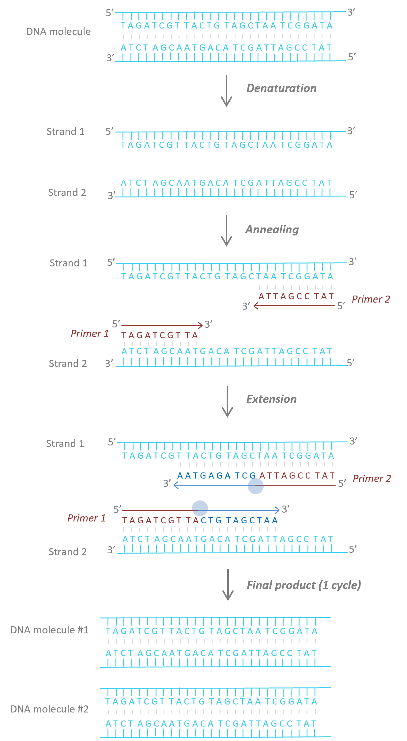
Fig. 5 PCR phases. i) Denaturation (92°-95°C): heat denatures DNA strands into single-stranded template DNA. ii) Annealing (55-65°C): primers bind to their complementary sequence on the single-stranded template DNA. iii) Extension (72°C): Taq polymerase (blue circle) extends the primers: new strands of DNA are now synthetized. At the end of each cycle of the three phases, the number of DNA molecules is doubled. The cycles are repeated between 30 and 40 times to obtain millions of DNA molecules.
Quantitative PCR (qPCR)
Quantitative PCR (qPCR) records the accumulation of DNA sequences in real time (thus sometimes called real time PCR) during amplification via the continuous measurement of a fluorescence signal incorporated into the amplified DNA. Most eDNA-based studies have shown a positive relationship between focal taxon abundance or biomass and eDNA concentration estimated using qPCR (Rourke et al. 2022). The two main chemistries for qPCR assays use either an intercalating dye, typically SYBR green (a fluorescent cyanine dye used as a nucleic acid stain), or a fluorescent probe (often TaqMan brand, specific oligonucleotide probes with a fluorophore at its 5’-end and a quencher at its 3’-end). SYBR-based assays are typically lower cost compared to probe-based assays, but have lower specificity due to the lack of a third primer-probe between the forward and backward primers, and cannot be multiplexed (where primer pairs for multiple species are run in the same reaction, potentially saving reagents and sample/template DNA). Multiplexed probe-based assays must have compatible fluorophore channels (specific to a qPCR platform) and quenchers.
SYBR green binds to double stranded DNA during amplification in a non-specific way whereas the Taqman probe chemistry relies on a 20bp sequence (probe) that specifically binds to the desired DNA fragment. During extension using the probe, the fluorophore and the quencher are cleaved out allowing the emission of the fluorescence signal. Thus, the quantification of DNA using those chemistries is made possible by the continuous proportionality between the level of fluorescence and the amount of amplified DNA. As the fluorescence is directly proportional to the number of amplicons produced during amplification, the fluorescence follows a typical amplification curve over the amplification cycles (Fig. 6 A). During the first cycles the fluorescence emission cannot be distinguished from the background noise (too few amplicons; PHASE 1), after which fluorescence level exceeds the background noise (detection threshold) and linearly increases (PHASE 2) to reach a plateau during which very few new amplicons are produced (PHASE 3). The number of cycles to pass the detection threshold (Ct or Cq value - synonyms) is inversely proportional to the number of copies of template DNA originally present in the sample. The unknown concentration of the extracted DNA sample is calculated using a linear regression of known concentration standards (“standard curve” or “calibration curve”, Fig. 6 B). The standard curve is made from serial dilutions (2 to 10-fold) of a positive control (known concentrations of DNA of the species of interest). Synthetic DNA is preferred to DNA extracted from tissue or blood, as it has a fixed number of base pairs and can be quantified in terms of copies per volume (Langlois et al. 2021). When using extracted DNA, it is typically best to verify the identity of the sample through PCR and Sanger sequencing if possible.
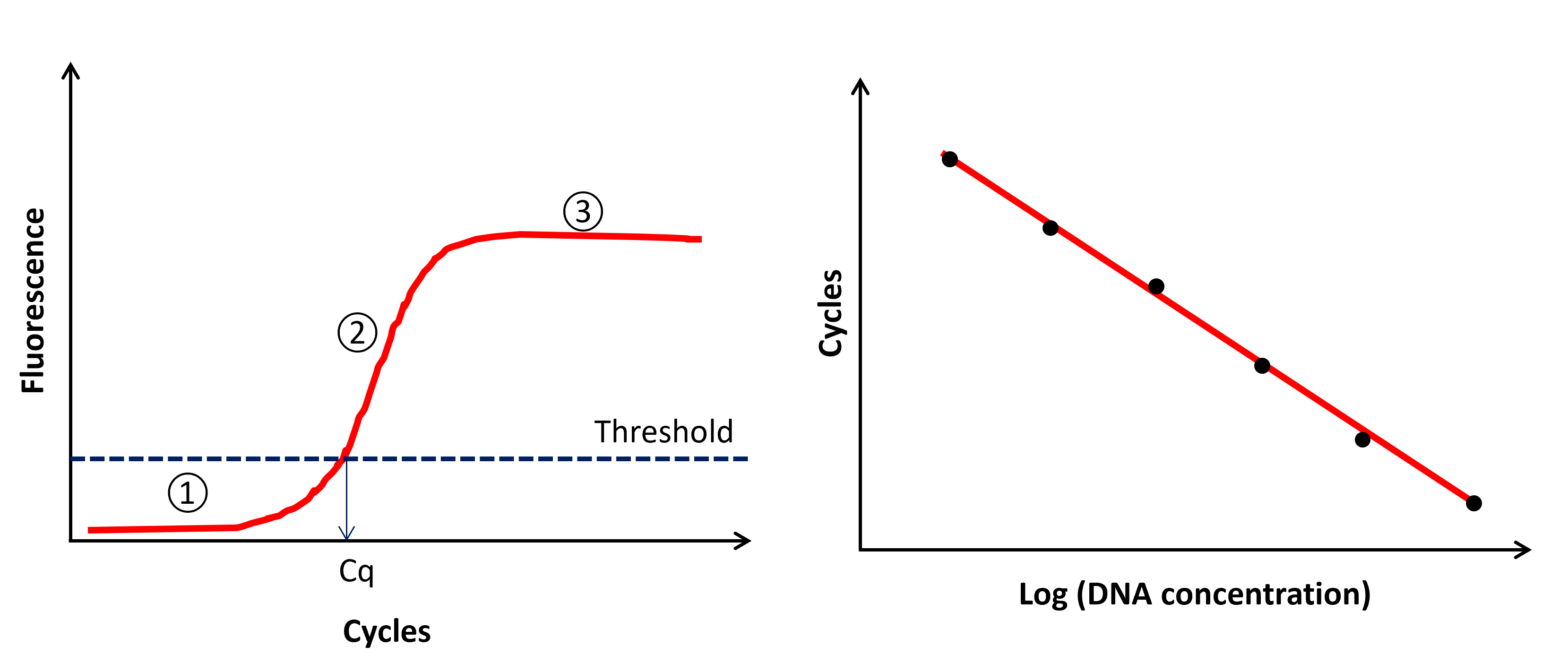
Fig. 6 A) Fluorescence emission across cycles. Phase 1 is defined by fluorescence emission below the background noise (threshold of fluorescence). Phase 2 is defined by a linear increase of the fluorescence emission and phase 3 by a plateau of fluorescence. Cq is the number of cycle to reach the threshold of fluorescence (i.e. fluorescence above background noise). B) Standard curve results. Each dot represents a concentration standard of the dilution series.
Quantitative PCR assay performance is evaluated using four metrics \(R^2\), PCR efficiency (\(E\)), Limit of Detection (LOD) and Limit of Quantification (LOQ).
\(R^2\) indicates how well the replicates fit on the standard curve (linearity). Usually we aim for \(R^2 > 98\%\).
PCR efficiency (\(E\)) is calculated using the formula:
When \(E=100\%\), this indicates that the amount of DNA product doubles with each cycle (MIQE guideline, Bustin et al. 2009). Lower values of E result from poor amplification, for example due to non-optimal qPCR mix or cycling conditions, secondary structure or primer dimers that affect primer-template annealing (poor amplification). \(E >100\%\) generally reveals polymerase inhibition, either by excessive initial DNA concentration or the presence of inhibitors in the sample (i.e. substances that negatively impact amplification because they interact with DNA or the polymerase). A value that exceeds 100% means that even if more DNA template is present in the reagent mixture, the Cq values might not shift accordingly which flattens out the efficiency plot, (lower slope and \(E > 100\%\)). We typically aim for \(90\% < E < 110\%\).
Limit of Detection (LOD) and Limit of Quantification (LOQ). The definition of the LOD and LOQ vary among authors (Forootan et al. 2017; Klymus et al. 2020a; Hunter et al. 2017; Brys et al. 2021) but the take home messages are:
#. LOD is a threshold above which it is possible to assess presence/absence of the target species with confidence even at low numbers of DNA copies, #. LOQ is the threshold over which we can confidently quantify the concentration of the target species (lowest value of the linear dynamic range of the standard curve). LOQ can only be equal to or greater than LOD. #. The LOD and the LOQ can be assessed using various methods, including discrete threshold methods and modelling methods (Klymus et al. 2020a; Hunter et al. 2017).
Example of discrete threshold method (Kubista 2014; Klymus et al. 2020a): The LOD is the lowest concentration of standard that produces at least 95% positive replicates (notemplate and negative controls must be blank). The LOQ is the lowest concentration of a standard whose coefficient of variation (relative standard deviation of the mean) value is below 35%. It is common to detect target DNA at concentrations below the LOD when multiple technical replicates are used: those detections should be interpreted with lower confidence. To overcome the issue of multiple technical replicate variability, Hunter et al. (2017) consider the LOD as “the lowest amount of analyte that can be both detected and distinguished from the concentration plateau” of the standard serial dilution.
We also strongly recommend reading Thalinger et al. (2021b) to understand how to interpret and fully appreciate the results of qPCR and get robust species-specific assays. The authors provide a five level validation scale specifically for the use of qPCR in eDNA studies. Validation is typically specific to your primer set, qPCR machine model, qPCR consumables, and even the target region. It is critical that one tests assays from the literature before extensive use.
Digital PCR (dPCR)
Digital PCR (dPCR) is an emerging technique for highly precise quantification of nucleic acids through partitioning into many simultaneous reactions. It is generally considered to be more sensitive than PCR followed by gel electrophoresis/Sanger sequencing and qPCR (Mao et al. 2019). dPCR involves separating a PCR reaction into thousands of microfluidic-scale volume partitions, where each partition can have no template DNA present, one copy of template DNA, or many copies of template DNA depending on the concentration in the original sample. When the number of partitions greatly exceeds the number of copies of template DNA, most partitions theoretically will contain zero or one copies of template. Therefore, the number of positive partitions is equal to the number of copies of template target DNA, and any stochasticity and droplets with multiple copies can be corrected for with Poisson statistics (Zhu et al. 2015). Advantages of dPCR include providing absolute quantification without a standard curve through Poisson distribution corrected binary counts of template DNA, high accuracy and sensitivity (which also corresponds to low sample volume requirements, which is often highly beneficial for eDNA samples), and better resistance to PCR inhibitors due to being an end-point assay with independence on amplification efficiency between partitions (Zhut et al. 2015, personal communication, Bio-Rad). However, inhibition can still affect dPCR results (Chen et al. 2023), and should therefore always be investigated regardless of the technology used. Weaknesses of the technique includes typically higher costs of the instrumentation and reagents than qPCR, narrow dynamic range (with a low maximum template DNA concentration), and potentially lower throughput. dPCR assays use the same primer/probe that qPCR assays use, so qPCR assays can be quickly adapted to dPCR. However, polymerase master mixes are typically specific to a dPCR platform, and cannot be interchangeably used. Most dPCR platforms are also suitable for multiplexing which can save cost of consumables and time. As a relatively new technology, dPCR platforms and best practices are constantly and quickly evolving.
Partitioning can be achieved through two main categories of methods. Chip-based methods use microfluidic arrays on chips or plates. With chip dPCR, the reaction mixture is pumped into nanoliter-scale chambers (between 10,000 to 40,000) through microfluidic forces (e.g. capillary action, centrifugal forces). The reactions then undergo thermocycling. The resulting fluorescence is then read in a way similar to pixels on a monitor (Zhang et al. 2015). Chip dPCR (cdPCR) systems include Standard BioTools’ (formerly known as Fluidigm) BioMark HD system, ThermoFisher’s QuantStudio Absolute Q Digital PCR system, and Qiagen’s QIAcuity system (Standard BioTools Inc, Thermo Fisher Scientific Inc, Qiagen N.V, Dong, Ming et al., 2015).
Droplet digital PCR (ddPCR) is based on water-oil emulsion droplet technology: a DNA sample is randomly partitioned into up to 20,000 individual droplets which are then independently amplified by conventional PCR enabling detection and quantification of very low amounts of DNA (Nathan et al. 2014) (Fig. 7). Concentration of target DNA is then determined by the fraction of positive droplets at the end of the PCR reaction (Fig. 7), whereas qPCR fluorescence is measured in real-time. ddPCR has several advantages compared to qPCR (Mauvisseau et al. 2019; Kamel et al. 2021; Doiet al. 2015a; Doiet al. 2015b): 1) ddPCR provides absolute quantification without the use of a standard curve; 2) ddPCR has a lower sensitivity to inhibitors (e.g. humic substances) present in environmental samples; and 3) the quantified concentration can be more accurate than qPCR especially at low concentration. As of April, 2024, Bio-Rad is the only supplier of ddPCR systems (see references).

Fig. 7 ddPCR workflow and graphic output.
Loop-mediated isothermal amplification (LAMP)
Notomi et al. 2000) but was first applied to single-species detection in eDNA-based studies only a few years ago (Davis et al. 2020; Williams et al. 2017; Kamel et al. 2021; Vythalingam, Hossain, and Bhassu 2021). LAMP involves using polymerases isolated from thermophilic bacteria (Milligan et al. 2018) that can cycle through dsDNA denaturation and amplification in isothermal conditions (i.e. does not require the multiple steps at different temperatures used in conventional PCR). In LAMP, four to six primers are used to target six to eight regions of a target sequence of DNA. These consist of a pair of external primers (which are similar to conventional PCR primers), a pair of internal primers, one complementary to the sense strand slightly downstream of the external primers, and the other complementary to an inner region of the target DNA sequence, and finally an optional pair of loop primers, which target regions between the two internal primer targets (Fig. 8). For more information on the mechanisms of LAMP, refer to: https://youtu.be/L5zi2P4lggw and Fig. 9.
LAMP has advantages and disadvantages over PCR, qPCR, or ddPCR. Unlike PCR-based detection methods, LAMP is isothermal and does not require temperature cycling. This can greatly reduce the cost and size of apparatus and power needed, facilitating its use for on-site detection and citizen science-based approaches. LAMP is highly tolerant of inhibitory salts and physicochemical conditions common to eDNA samples. Yield and speed are typically superior to PCR based methods and can be visible to the naked eye through turbidity induced by magnesium pyrophosphate precipitation or pH change (Soraka et al. 2021, Mori et al. 2001, Tanner et al. 2015). Due to the larger number of primers, LAMP is typically thought to be more specific than non-probe-based qPCR (probes significantly raise the cost of qPCR). LAMP primer design also does not require gradient PCR testing. However, LAMP products are complex mixes of concatemers with the target sequence, and not suitable for downstream applications without further processing (Sahoo et al. 2016). LAMP is also difficult to multiplex, the primers are difficult to design manually, and LAMP reagents are more costly due to lower economy of scale. Nevertheless, the use of LAMP in biomedical and environmental detection has received significant recent attention (Seki et al. 2018; Ganguli et al. 2020).

Fig. 8 Primers used in LAMP. The boxes on the lines represent different parts of the target sequence. Striped boxes are complementary to solid boxes of the same colour. Free floating boxes are primers, and their colour and solid/striped fill-in indicates which part of the target sequence they are from. Primers are approximately 20 bp long.

Fig. 9 LAMP process.
Inhibition and Internal Positive Controls (IPC)
eDNA samples often contain compounds that inhibit PCR or impede fluorescence (McKee et al. 2015) resulting in potential false negatives or lower detected concentrations. Inhibitors include compounds from decaying organic materials, such as tannins, humic acids, and fulvic acids, excreted compounds, such as bile salts, complex polysaccharides, and urea, and intra-cellular/intra-tissue compounds, such as collagen, heme, and calcium ions (Hunter et al. 2019, Rådström et al. 2004). A high concentration of non-target DNA, particularly when there are few mismatches between primers and templates is also a potential inhibitor, particularly for qPCR (Latham et al. 2023). Environmental conditions such as pH can also result in PCR inhibition. Inhibition is typically a significant issue when target DNA concentrations are low (below 10-100 copies/µL).
Best practice in eDNA inhibition involves optimizing sampling protocols in the study design phase, using an internal positive control (IPC), using inhibition mitigation methods on samples where inhibition has been detected, and properly reporting inhibition. During study design, sites that have lower chances of inhibition should be selected when possible. Common indicators of potential inhibition include high turbidity, darker water (which is an indicator of humic acid compounds), the smell of decaying vegetation (both macrophytes and algal blooms), and a shallow lakebed with finer particles. Additionally, sampling should be avoided after immediate precipitation (Chen et al. 2023). For sites where inhibition is more likely, larger pore size filters (5-10 micron) may reduce clogging and co-extraction of inhibitor compounds (Brown et al. 2025).
The effect of inhibition can be assessed using an IPC (see Klymus et al. 2020b for more details). This typically involves the addition of a low concentration (approximately 100 copies/µL) of foreign DNA (DNA that is unlikely to be present in your sampled site; e.g. from a species endemic to a different continent) and a matching assay which must be multiplexed with your target assay to both your eDNA samples and no-template controls. In qPCR, non-amplification, a Cq value shift of over three cycles, or a much lower concentration of your IPC assay in your eDNA samples compared to your NTC indicates inhibition (Hartman et al. 2005). In dPCR, droplet or partition fluorescence amplitudes of the IPC assay that are significantly below the positive control indicate inhibition, forming a ‘rain’ like pattern of fluorescence amplitudes on the dPCR software (Chen et al. 2023). IPCs must be validated through testing with your assay, as multiplexing may be a source of competitive inhibition in itself. When inhibition is suspected, IPCs should be used on all samples.
When inhibition is detected, methods for reducing it include diluting the eDNA sample with buffer or dH2O, altering PCR conditions (by adding bovine serum albumin or BSA, using a more inhibitor-resistant polymerase, changing cycle count, step length, or ramping time) or inhibitor removal (through a commercial kit, re-extraction, or ethanol precipitation) (Chen et al. 2023). All methods come with their own risks, such as DNA loss with dilution or inhibitor removal, or false positives with changing PCR parameters (Goldberg et al. 2016). When the IPC indicates inhibition in negative samples, we recommend diluting the eDNA sample with dH2O between 1:10 and 1:50, and adding 0.1 µg/µl of BSA (Chen et al. 2023, Wang et al. 2017, Kreader 1996). Inhibition mitigation is not necessary in positive samples unless quantification is required. In that case, dilute the sample and add BSA as with a negative sample, and back-multiply by your dilution factor in your concentration calculations.
Inhibition is a complex topic that requires iterative, trial and error-based testing for each study. There is currently no consensus on mitigating the negative effects of inhibition in eDNA. We recommend reporting the method you used to detect and address the issue of inhibition in detail, and indicating which samples had inhibition detected (particularly negative samples). We also recommend adapting your sampling scheme based on your results, if possible.